Copula-Based Dependence Measures for Under-Five Mortality Rate in Rwanda
Fidence Munyamahoro
DOI10.21767/2471-8041.100034
Fidence Munyamahoro*
Department of Actuarial Science, University of Lausanne, Switzerland
- *Corresponding Author:
- Fidence Munyamahoro
Department of Actuarial Science
University of Lausanne, Switzerland.
Tel: +41216921111
E-mail: fidence.munyamahoro@unil.ch
Received Date: May 19, 2016; Accepted Date: November 23, 2016; Published Date: November 28, 2016
Citation: Munyamahoro F. Copula-Based Dependence Measures for Under-Five Mortality Rate in Rwanda. Med Case Rep. 2016, 2:3. doi: 10.21767/2471-8041.100034
Abstract
The risk of a child dying before completing five years of age is still highest in sub-Saharan Africa region. In this paper, we used the copula based dependence to investigate the association between the under-five mortality rate and Gross Domestic Product in Rwanda from 1981 to 2015. The copula has for a long time been recognized as a powerful tool for modeling dependence between two random variables. The Archimedean copulas were applied to capture the non-linearity in the dependence structure between those two vectors. Our findings showed that after 1994, the under-five mortality rate in Rwanda diminished steadily from 300 up to 42 per 1000 lives in 2015. Our analysis showed that under-five mortality rate is inversely proportional to the Gross Domestic Product. Unfortunately, it is not obvious to predict the future under-five mortality rate according to the Gross Domestic Product because it changes yearly according to the political measures of country. In this paper, we considered two Archimedean copulas namely Gumbel and Clayton.
Keywords
Under-five mortality rate; Gross domestic product; Dependence measures; Gumbel and Clayton copula; Kendall’s tau
Introduction
The risk of death of children under-5 years is still very high in sub-Saharan Africa region. Children in sub-Saharan Africa are more than 14 times more likely to die before the age of five than children in developed regions, WHO [1]. A child’s risk of dying is highest in the neonatal period, the first 28 days of life. Safe childbirth and effective neonatal care are essential to prevent these deaths. The poverty is main factor which makes the number of children dying per thousand lives in this region be very high. Under-five mortality is still high in low and middle income countries; in this paper, we used a copula approach to measure the dependence between under-five mortality rate and gross domestic product (GDP) in order to investigate the level of effect of GDP to the mortality. The higher GDP is, the lesser is the mortality rate under-five.
The copula is powerful tool for dependency structure; it is a good approach for non-linearly correlated variables. The Pearson correlation coefficient was developed basically for measuring the correlation and addresses only linear dependence, this is meaningful measure of dependence and it is very flexible with the elliptical distributions. The draw- back of linear correlation coefficients is that out of elliptical distributions, the usage may mislead to the good conclusion. However, an innovative approach, the so-called copula method, provides the ability to couple any marginal distributions and overcome the above linear correlation weakness.
The word “copula” derives from the Latin noun for a “link” or “tie” that connects two different things and concept of copula in sciences was introduced by Sklar and has for a long time been being recognized as a powerful tool for modeling dependence between two random variables. In this article the Archimedean copulas were used for modelling the concordance measures: Kendall’s tau and spearman’s rho for mortality rate under-5 years in Rwanda in the period of 1981-2015.
Materials and Methods
The under-five mortality rate is a key indicator of child wellbeing and It is also a key indicator of the coverage of child survival interventions and, more broadly, of social and economic development of a country. It is important to use sound statistical methods to determine which factors are strongly associated with child mortality which in turn will help inform the design of intervention strategies. This paper focused on Rwanda, the under-five mortality rate in Rwanda as well as its GDP. The Table 1 summarizes the situations from 1981 to 2015.
| N | Minimum | Maximum | Mean | Std. Deviation | Skewness | Kurtosis | |||
|---|---|---|---|---|---|---|---|---|---|
| Statistic | Statistic | Statistic | Statistic | Statistic | Statistic | Std. Error | Statistic | Std. Error | |
| Gross Domestic Product in billion $ | 35 | 1.2 | 8.5 | 3.048 | 2.146 | 1.432 | 0.398 | 0.721 | 0.778 |
| Number of death per 1000 | 35 | 42 | 300 | 146 | 64.344 | 0.128 | 0.398 | -0.236 | 0.778 |
Table 1: Descriptive statistics.
In last 35 years (from1981 to 1015) the maximum and minimum under-five mortality rate in Rwanda are 300 and 42 respectively while the maximum and minimum of GDPs are respectively 8.5 and 1.2 billion$. This maximum death rate appeared in 1994 and in this period (1994 and 1995), minimum GDP (1.2$ billions) appeared. It is obvious to conclude that the under-five mortality rate is inversely proportional to the GDP. The seventh column contains the skewness coefficients, and is positive for both under-five mortality rate and GDP. Positive skewness indicates that the tail on the right side is longer or fatter than the left side. Standard errors are relatively small. The following figure shows scatter plot of under-five mortality rate vs the GDP in Rwanda from 1981 to 2015 (Figure 1).

Figure 1: Scatter plot of under-five mortality vs gross domestic product in Rwanda from 1981 to 2015.
From the above figure, the under-five mortality rate is very high when the GDP is small. In Rwanda there is clear reduction of under-five mortality rate after 1994 and the GDP also increased significantly. In 2015, the under-five mortality rate is 42 per thousand lives, this is good achievement but it is still high compared to European countries where the rate was 11 per 1000 lives in 2015. GDP measures the nations, total output of goods and services; it should help to better relate individual household and personal income. It enables policymakers and central banks to judge whether the economy is contracting or expanding. In this paper, we investigated the impact of GDP to the under-five mortality and it is very clear that the death reduces according to increasing of GDP. The Table 2 shows how those two variables have the strong negative relationship between them (Figure 2).
| Number of death per 1000 | Gross Domestic Product in billion $ | |||
|---|---|---|---|---|
| Kendall's tau_b | Number of death per 1000 | Correlation Coefficient | 1 | -0.801** |
| N | 35 | 35 | ||
| Gross Domestic Product in billion $ | Correlation Coefficient | -0.801** | 1 | |
| N | 35 | 35 | ||
| Spearman's rho | Number of death per 1000 | Correlation Coefficient | 1 | -0.905** |
| N | 35 | 35 | ||
| Gross Domestic Product in billion $ | Correlation Coefficient | -0.905** | 1 | |
| N | 35 | 35 |
Table 2: Correlations.

Figure 2: Cumulative Survival function for under-five mortality in Rwanda from 1981 to 2015.
From this table, the Kendall’s tau is -0.801 and Spearman’s rho is -0.905. These values are much closed to -1. That is the perfect negative correlation between these two variables. The GDP of developed countries is high which makes the under-five mortality to be small. The GDP of sub-Saharan Africa region is very low compared to developed countries; this is the main reason-why the under-five mortality rate is too high in this region. It is obvious to say that under-five mortality is a factor that is associated with the well-being of a population and it is taken as an indicator of health development and socioeconomic status.
Survival Analysis
Survival function
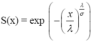
Let T be a continuous random variable with probability density function f (t) and cumulative distribution function 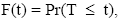 which gives the probability that the event has occurred by duration t. the survival function or reliability function is
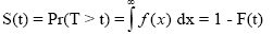 which gives the probability of being alive just before duration t. Every survival function S(t) is monotonically decreasing, i.e.
  for all u > v . The following figure shows the survival function of the under-five mortality rate in Rwanda (Figure 2).
Hasard function
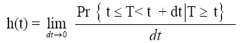
An alternative characterization of the distribution of random variable T is given by the hazard function, or instantaneous rate of occurrence of the event, defined as:
Hazard proportional model is useful to analyze the risk of death given the explanatory variables. The good important feature for Cox proportional model is that it could estimate the relationship between the hazard rate and explanatory variables without having to make assumptions about the shape of the baseline hazard function (Figure 3).

Figure 3: Cumulative Hasard function in terms of mean covariates for under-five mortality in Rwanda. From 1981 to 2015.
The hazard function is neither a density nor a probability. However, it may be the probability of failure in an infinitesimally small time-period between t and t + dt given that the subject has survived till time t. In this sense, the hazard is a measure of risk: the greater the hazard between times t1 and t2, the greater the risk of failure in this time interval.
Kaplan Meier estimator
Survival analysis is the evaluation of how long individuals, who are endangered of certain health risk, will survive. Kaplan-Meier estimator is one of most frequently used survival analyses. It is also known as the product limit estimator, is a non-parametric statistic used to estimate the survival function from lifetime data. In medical research, it is often used to measure the fraction of patients living for a certain amount of time after treatment (Figure 4).

Figure 4: Kaplan Meier survival functions.
The probabilities shown are called Kaplan-Meier survival probabilities and have a unique interpretation. The survival probabilities are conditional ones and indicate the probability of experiencing the primary endpoint beyond a certain length of time. Curves that have many small steps usually have a higher number of participating subjects, whereas curves with large steps usually have a limited number of subjects.
Marginal Distributions
Introduction
A study of mortality law was introduced by De Moivre. De Moivre himself did not consider his law (he called it a “hypothesis”) to be a true description of the pattern of human mortality. Instead, he introduced it as a useful approximation when calculating the cost of annuities. From that period, the different suggestions have been made to formulate the mathematical formulas of law of mortality, of which the Gompertz [2] is the most famous. The many formulas are based on age and accordingly, three different periods are considered: infant mortality or mortality during childhood (this is rapid decrease of mortality during the first few years of life), mortality at the middle ages (where the deaths are mainly due to accidents) and mortality at the adult ages (is the almost geometric increase of mortality with age). Common known functions to model the mortality law are Gompertz, Weibull, Inverse-Gompertz, Inverse-Weibull, Gamma and lognormal. The Gompertz’s law fits observed mortality rates very well at the adult ages. Jacques and Carriere [3] pointed out that for certain parameter values the Weibull has a decreasing force of mortality, and so it seems that this may be a plausible model for early childhood where mortality rates are decreasing. In this paper, we used the Weibull distribution to model the under-five mortality rate and it seems to be the appropriate one to our dataset.
Weibull model
The Weibull survival function is given by:
 (1)
(1)
where λ > 0 is a location parameter and σ > 0 is a dispersion parameter. The cumulative distribution function is given by:
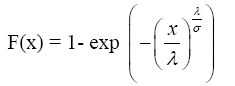 (2)
(2)
Hence the density function is given by:
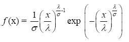
The force of mortality is: 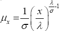 when
when then the mode of the density is 0 σ λ and μx is a non-increasing function of x.
P-P plot and Q-Q plot: In statistics, a P-P plot (probabilityprobability plot or percent-percent plot) is a proba- bility plot for assessing how closely two data sets agree, which plots the two cumulative distribution functions against each other. P-P plots are vastly used to evaluate the skew- ness of a distribution. A P-P plot can be used as a graphical adjunct to a test of the fit of probability distributions with additional lines being included on the plot to indicate either specific acceptance regions or the range of expected departure from the line. P-P plot is used in this paper to test the goodness of fit of weibull distribution to our data base (Figure 5).

Figure 5: Weibull P-P plot for under-five mortality rate in Rwanda from 1981 to 2015.
Another useful probability plot is Q-Q. The Q-Q plot, or quantilequantile plot, is a graphical tool to help us assess if a set of data plausibly came from some theoretical distribution such as a Normal or exponential. A Q-Q plot (“Q” stands for quantile) is a probability plot, which is a graphical method for comparing two probability distributions by plotting their quantiles against each other. The points plotted in a Q-Q plot are always non-decreasing when viewed from left to right. Another common use of Q-Q plots is to compare the distribution of a sample to a theoretical distribution (Figure 6).

Figure 6: Weibull Q-Q plot for under-five mortality rate in Rwanda from 1981 to 2015.
From the Figure we can conclude that our data for under-five mortality are normally distributed. The test of normality is performed in section 6 (Figure 7).

Figure 7: Weibull Q-Q plot Gross Domestic in Rwanda from 1981 to 2015.
It seems to us that a distribution more skewed to the right would be a better fit, is that right (right skewness) so that our data of GDP Product is not normally distributed. We will conclude about this in normality test in section 6. On appendix, there is the detrended Q-Q plot of GDP.
Kernel density estimation for GDP
A kernel is a non-negative, real-valued, integrable function (sometimes also called summable function) K(.) satisfying the following two requirements:
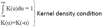 (3)
(3)
Due to our data for GDP, we use a kernel density to promote the continuity nature in the underlying random variable. The intuition of choosing kernel density for GDP is relatively straight forward. Kernel density estimation is a fundamental data smoothing problem where inferences about the population are made, based on a finite data sample. It is a non-parametric way to estimate the probability density function of a random variable. The kernel distribution may be a good approach for analyzing the GDP. Delfin and John [4] used kernel distribution to analyse GDP data, Jorge Saba and Arbache [5] used it for GDP per capital and Daniel et al. [6], Falko Juessen [7] also used the Gaussian kernel density for GDP data. In this paper, we used the Gaussian kernel density to model the GDP in Rwanda from 1981 to 2015 (Figure 8).

Figure 8: Kernel density estimation for real GDP growth per cent in Rwanda from 1981 to 2015. The blue color indicates the KDE curve and the red one indicates the Gaussian curve.
Consider a random sample, X = {x1, x2, ..., xn}, from an unknown population with density f, a nonparametric estimate of this density is given by:
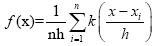 (4)
(4)
Where K(.) is the Gaussian kernel function and h is the smoothing (or scaling) parameter and K(x) usually chosen as a symmetric probability density function satisfying the condition [8]. The Gaussian or Normal kernel is given by:
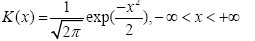 (5)
(5)
By putting (5) in (4), we get the Gaussian kernel density estimate
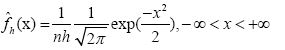 (6)
(6)
Maximizing likelihood, choose 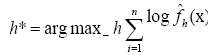 .The ML estimate of h is degenerate since it yields
  a practical alternative is to maximize the pseudo- likelihood computed using leave-one-out cross-validation.
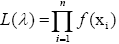
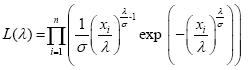
Maximum likelihood estimation
The maximum likelihood function is given by:
 for our case, n = 35 years and by using (2), we get:
To optimize this function, a logarithmic approach is the simple way; the maximum log likelihood function is given by:
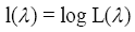
Hence
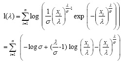 (7)
(7)
By maximizing the equation (7), we get the estimates of parameters. Using our dataset, the MLE estimates are shown in the next table (Table 3).
| Variables | Average x¯ | Estimate | Estimate |
|---|---|---|---|
| Death rate (per 1000) | 146 | 164.65 | 66.15 |
| Mkle maximum kernel likelihood estimate | |||
| GDP (in billion $) | 3.0486 | 3.0486 | |
Table 3: Parameter estimates.
The average of under-five mortality rate in Rwanda in last 35 years is 146 per thousand lives and average of GDP is 3.0486 billion$. The mode of under-five mortality rate in last 35 years in Rwanda is 164.65 and the bandwidth or smoothing (or scaling) parameter for GDP 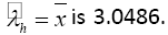 These estimate values can be used later to calculate the dependence coefficients.
Models of Dependence
Copula and its applications
The copula has for a long time been recognized as a powerful tool for modeling dependence between two random variables. This paper describes the copula-based prediction modeling which can be employed as a good alternative to the linear correlation-based modeling in different domains. Let F (x, y) denote the cumulative probability distribution of under-five mortality rate in Rwanda (X) and GDP (Y) and marginal distributions of X and Y be F1(x) and F2(y) respectively.
Let X and Y be continuous random variables with distribution functions F1(x) = Pr(X ≤ x) and F2(y) = Pr(Y ≤ y) respectively, the joint distribution function of X and Y is:
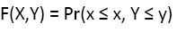
Then there exists a copula C such that F (X, Y) = C(F1(x), F2(y)). Conversely, for any distribution functions F1 and F2 and any copula C, the function F defined above is a two-dimensional distribution function with marginals F1 and F2 . Furthermore, if F1 and F2 are continuous, C is unique.
The copula C is the function mapping from [0, 1]2 to [0,1] such that for all x ∈ [0, 1], C(x, 0) = C(0, x) = 0 and C(x, 1) = C(1, x) = x For all a, b, c, d ∈ [0, 1] and a ≤ b, c ≤ d, VC ([a, b]X[c, d]) = C(b, d) − C(b, c) − C(a, d) + C(a, c) The function VC is called the C-volume of the rectangle [a, b][c, d].
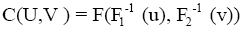
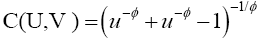
The copula function is very useful when dealing with vectors of random variables because it allows us to model the dependence between the variables separately from their marginals. Let apply probability transforms U = F1(x) and V = F2(y) to X and Y with U and V uniform random variables defined on [0, 1], there exists a bivariate copula function C(U,V ) such that:

If F1(x) and F2(y) are continuous then C (u, v) is unique otherwise C (u, v) is uniquely determined on range of F1(x) times range of F2(y). Given a joint distribution function F with continuous and invertible marginals F1 and F2 , as in Sklars Theorem it is easy to construct the corresponding copula:
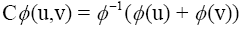
There are many families of copulas but in this paper, we only focus on Archimedean copula family with one parameter. The Archimedean copula family is popular due to its flexibility in modeling dependence. In our case, the Archimedean copula used to model the dependency between under-five mortality rate in Rwanda and GDP. Let φ be a twice-differentiable strictly decreasing function from [0, 1]to [0, ∞] such that φ(1) = 0 and φ−1 be generalized inverse of φ. The distribution function of Archimedean copula is given by:
 (8)
(8)
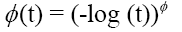
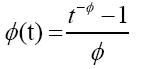
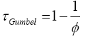
φ is called Archimedean generator. We focused on two Archimedean copulas named Gumbel and Clayton. The Gumbel and Clayton copula is associated respectively to the following generators:
 (9)
(9)
and
 (10)
(10)
With θ a positive parameter that controls the dependency among variables. By using the Gumbel’s generator (equation (9)) in (8), the Gumbel copula is given by:
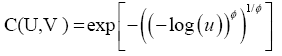 (11)
(11)
Similarly, by using (10) in (8), the Clayton copula is given by:
 (12)
(12)
Copula parameter estimation
The maximum-likelihood estimation of the copula parameters is based on the copula density. Parameter estimation using maximum-likelihood usually requires a parametric or nonparametric approximation of the marginal distributions of random variable. In this paper, we only consider the bivariate case. Hence the log likelihood function is given by:
 (13)
(13)
With U and V uniform random variables defined on [0, 1] and given by: U = F1(x) and V = F2(y), c(U, V ) is the second derivative of C(U, V ) with respect to U and V . Maximizing equation (13) we get the maximum likelihood estimator of parameter θ. The Table 4 contains the estimate parameters.
| Copula | Parameter |
|---|---|
| Gumbel Copula | 2.78 |
| Clayton Copula | 4.45 |
Table 4: Copula parameters estimate.
The estimates of the dependence parameter for Gumbel and Clayton copula are 2.78 and 4.45 respectively. These values are useful for calculating the tail dependence and correlation coefficients.
Copula- based dependence measures
The tail dependence coefficients as well as concordance measures: Kendall’s tau and spearman’s rho are good measures of dependency, especially to our database which is not appropriate to the linear correlation. The Kendall’s tau of two variables X and Y with C (U, V) the copula of bivariate distributions X and Y is given by:
In spite of this formula, Kendall’s tau for Archimedean copula can be expressed as one dimensional integral of the generator and its derivative as shown by Genest and MacKay [9]. Then, Kendall’s tau for Archimedean copula can be calculated by using the following formula:
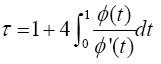 (14)
(14)
where φ is called an Archimedean generator. The Kendall’s tau for Gumbel copula is calculated by putting (9) in (14):
Similarly, by putting (10) in (14) we get the Kendall’s tau for Clayton copula.
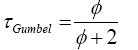
By using the results from Table 4, we can compute the value of Kendall coefficients (Table 5).
| Copula | Kendall's tau |
|---|---|
| Gumbel copula | 0.64 |
| Clayton copula | 0.69 |
Table 5: Kendall’s tau.
According to these generated results, there is a significant relationship between under- five mortality rate and GDP. τ (X, Y ), the Kendall’s tau for variables X and Y is considered as measure of monotonic dependence between those two variables. Nevertheless, this measure is invariant under monotone transformation and the drawback of linear correlation is that in general it is invariant under that transformation. Embrechts et al. [10] suggested that it is better to use Kendall’s tau and Spearman’s correlation than using linear correlation.
Statistical Tests
Normality test
The Kolmogorov-Smirnov test (K-S test or KS test) is a nonparametric test of the equality of continuous, onedimensional probability distributions that can be used to compare a sample with a reference probability distribution (one-sample KS test), or to compare two samples (two-sample KS test). The Kolmogorov-Smirnov statistic quantifies a distance between the empirical distribution function of the sample and the cumulative distribution function of the reference distribution, or between the empirical distribution functions of two samples. The Kolmogorov-Smirnov test can be modified to serve as a goodness of fit test. In the special case of testing for normality of the distribution, samples are standardized and compared with a standard normal distribution. The empirical distribution function Fn for n iid observations Xi is defined as:
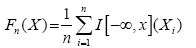
where  is the indicator function which is equal to 1 if Xi ≤ x and equal to 0 otherwise. The Kolmogorov-Smirnov statistic for a given cumulative distribution function
F (x) is:
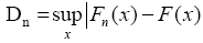
where supx is the supremum of the set of distances. The key observation in the Kolmogorov- Smirnov test is that the distribution of this supremum does not depend on the unknown distribution of the sample. i.e., if F (x) is continuous then the distribution of
 does not depend on F.
The normality tests are supplementary to the graphical assessment of normality. The main tests for the assessment of normality are Kolmogorov-Smirnov (K-S) test, Shapiro- Wilk test, Anderson-Darling test, Cramer-von Mises test, Jarque-Bera test, D’Agostino skewness test, D’Agostino-Pearson omnibus test, and Anscombe-Glynn kurtosis. The large number from any of these above tests supports the rejection of the null hypothesis. In this paper, we only used the Kolmogorov-Smirnov (K-S) test to test normality and the results are detailed in Tables 6 and 7 [11-20].
| Statistic | Std. Error | Bootstrap | |||||
|---|---|---|---|---|---|---|---|
| Bias | Std. Error | 95% Confidence Interval | |||||
| Lower | Upper | ||||||
| Number of death per 1000 | |||||||
| Mean | 146 | 10.876 | 0.25 | 9.69 | 125.23 | 163.18 | |
| 95% Confidence Interval for Mean | Lower Bound | 123.9 | |||||
| Upper Bound | 168.1 | ||||||
| 5% Trimmed Mean | 143.94 | 0.92 | 10.15 | 121.79 | 162.46 | ||
| Median | 155 | -0.57 | 9.7 | 124 | 170 | ||
| Variance | 4140.176 | -147.864 | 828.162 | 2490.115 | 5677.865 | ||
| Std. Deviation | 64.344 | -1.5 | 6.58 | 49.895 | 75.348 | ||
| Minimum | 42 | ||||||
| Maximum | 300 | ||||||
| Range | 258 | ||||||
| Interquartile Range | 97 | -6 | 24 | 35 | 129 | ||
| Skewness | 0.128 | 0.398 | -0.081 | 0.334 | -0.655 | 0.579 | |
| Kurtosis | -0.236 | 0.778 | 0.008 | 0.59 | -1.275 | 1.223 | |
| Gross Domestic Product in billion $ | |||||||
| Mean | 3.0486 | 0.36275 | -0.0208 | 0.3228 | 2.3944 | 3.8967 | |
| 95% Confidence Interval for Mean | Lower Bound | 2.3114 | |||||
| Upper Bound | 3.7858 | ||||||
| 5% Trimmed Mean | 2.8627 | -0.0145 | 0.3447 | 2.2048 | 3.7908 | ||
| Median | 2 | 0.022 | 0.2177 | 1.8 | 2.5433 | ||
| Variance | 4.606 | -0.09 | 1.154 | 2.211 | 6.735 | ||
| Std. Deviation | 2.14605 | -0.03942 | 0.28093 | 1.486 | 2.59523 | ||
| Minimum | 1.2 | ||||||
| Maximum | 8.5 | ||||||
| Range | 7.3 | ||||||
| Interquartile Range | 2.1 | 0.12 | 1.15 | 0.76 | 4.7 | ||
| Skewness | 1.432 | 0.398 | 0.046 | 0.406 | 0.574 | 2.452 | |
| Kurtosis | 0.721 | 0.778 | 0.362 | 1.588 | -1.317 | 5.701 | |
Table 6: Kolmogorov- Smirnov statistic.
| Kolmogorov- Smirnov | Shapiro- Wilk | |||||
|---|---|---|---|---|---|---|
| Statistic | df | Sig. | Statistic | df | Sig. | |
| Number of death per 1000 | 0.147 | 35 | 0.053 | 0.958 | 35 | 0.203 |
| Gross Domestic Product in billion $ | 0.297 | 35 | 0 | 0.75 | 35 | 0 |
Table 7: Tests of Normality.
The generated Kolmogorov-Smirnov table contains the descriptive statistics of both under-five mortality rate and GDP in Rwanda from 1981 to 2015. The bootstrap of 100 samples also was performed.
Refer to the generated above table, the Kolmogorov-Smirnov statistics are 0.147 and 0.297 for under-five mortality rate and GDP respectively. The corresponding P-values are .053 and .000 for respectively under-five mortality rate and GDP. Hence the under-five mortality rates are normally distributed while the GDPs are not. These results are not contrary to those found in section 3 about P-P and Q-Q plot [21-25].
Chi-square test
We would like to test whether there is a significant relationship between the under-five mortality rate and GDP. Previous generated output (kendall and spearman coefficient) showed that there is a strong negative relationship between those two variables. Using Chi-square test we can either reject or accept the hypothesis which states that there is a significant relationship between those variables (Table 8).
| Chi-Square Tests | ||||||||
|---|---|---|---|---|---|---|---|---|
| Value | df | Asymp. Sig. (2-sided) | Monte Carlo Sig. (2-sided) | |||||
| Sig. | 99% Confidence Interval | |||||||
| Lower Bound | Upper Bound | |||||||
| Pearson Chi-Square | 685.417 | 660 | 0.239 | 0.350 | 0.227 | 0.473 | ||
| Likelihood Ration | 199.647 | 660 | 1 | 1.000 | 0.955 | 1 | ||
| Fisher's Exact Test | 1204.207 | 1.000 | 0.955 | 1 | ||||
| Linear-by-Linear Association | 24.692 | 1 | 0 | 0.000 | 0 | 0.045 | ||
| N of Valid Cases | 35 | |||||||
| Bootstrap for Symmetric Measures | ||||||||
| Value | Bootstrap | |||||||
| Bias | Std. Error | 95% Confidence Interval | ||||||
| Lower | Upper | |||||||
| Nominal by Nominal | Phi | 4.425 | -0.653 | 0.211 | 3.338 | 4.139 | ||
| Cramer's V | 0.943 | 0.019 | 0.023 | 0.918 | 1 | |||
| Interval by Interval | Pearson's R | -0.852 | -0.007 | 0.037 | -0.933 | -0.774 | ||
| Ordinal by Ordinal | Spearman Correlation | -0.905 | 0.01 | 0.061 | -0.98 | -0.722 | ||
| N of Valid Cases | 35 | 0 | 0 | 35 | 35 | |||
| Symmetric Measures | ||||||||
| Value | Asymp. Std. Error a | Approx. Tb | Approx. Sig. | Monte Carlo Sig. | ||||
| Sig. | 99% Confidence Interval | |||||||
| Lower Bound | Upper Bound | |||||||
| Nominal by Nominal | Phi | 4.425 | 0.239 | 0.290c | 0.173 | 0.407 | ||
| Cramer's V | 0.943 | 0.239 | 0.290c | 0.173 | 0.407 | |||
| Interval by Interval | Pearson's R | -0.852 | 0.035 | -9.357 | 0.000d | 0.000c | 0 | 0.045 |
| Ordinal by Ordinal | Spearman Correlation | -0.905 | 0.051 | -12.2 | 0.000d | 0.000c | 0 | 0.045 |
| N of Valid Cases | 35 | |||||||
Table 8: Chi-Square test statistics and bootstrap for symmetric measures.
The P-value is 0.239 which is greater than 0.05 so that we fail to reject the null hypothesis, thus at 95% level of significance, we can conclude that there is a significant relationship between under-five mortality rate and GDP. The pearson correlation is -0.852 and Spearman correlation is -0.905, both values are closed to -1. hence there is a strong negative relationship between under-five mortality rate and GDP. The more GDP increases the more under-five mortality rate diminishes [25-30].
Conclusion
This paper deals with association between under-five mortality rate and GDP in Rwanda from 1981 to 2015. We used parametric correlation coefficient (Pearson) and non-parametric correlation coefficients (Kendall and Spearman) to investigate the relationship between those two variables. The Chi-square test showed that there is a relationship between under-five mortality rate and GDP. Most of our results focused on relationship and supported the ideal that the more is the GDP, the lesser is under-five mortality rate.
Appendix
1. Detrended Weibull PP and QQ plot (Figure 9 and 10).

Figure 9: Detrended P-P plot of under-five mortality rate.

Figure 10: Detrended QQ plot of gross domestic product.
2. Kaplan Meier survival and hazard function (Figure 11 and 12).

Figure 11: Kaplan Meier log survival function.

Figure 12: Kaplan Meier Hazard function.
3. Kaplan Meier survival analysis (Table 9 and 10).
| Survival Table | |||||
|---|---|---|---|---|---|
| Time | cumulative proportion surviving at the time | N of cumulative Events | N of Remaining cases |
||
| Estimate | Std error | ||||
| 1 | 42.000 | 0.971 | 0.029 | 1 | 34 |
| 2 | 44.000 | 0.943 | 0.039 | 2 | 33 |
| 3 | 48.000 | 0.914 | 0.047 | 3 | 32 |
| 4 | 52.000 | 0.886 | 0.054 | 4 | 31 |
| 5 | 58.000 | 0.857 | 0.059 | 5 | 30 |
| 6 | 64.000 | 0.829 | 0.064 | 6 | 29 |
| 7 | 71.000 | 0.800 | 0.068 | 7 | 28 |
| 8 | 78.000 | 0.771 | 0.071 | 8 | 27 |
| 9 | 88.000 | 0.743 | 0.074 | 9 | 26 |
| 10 | 99.000 | 0.714 | 0.076 | 10 | 25 |
| 11 | 111.000 | 0.686 | 0.078 | 11 | 24 |
| 12 | 124.000 | 0.657 | 0.080 | 12 | 23 |
| 13 | 139.000 | 0.629 | 0.082 | 13 | 22 |
| 14 | 149.000 | 14 | 21 | ||
| 15 | 149.000 | 0.571 | 0.084 | 15 | 20 |
| 16 | 152.000 | 16 | 19 | ||
| 17 | 152.000 | 0.514 | 0.084 | 17 | 18 |
| 18 | 155.000 | 18 | 17 | ||
| 19 | 155.000 | 0.457 | 0.084 | 19 | 16 |
| 20 | 157.000 | 0.429 | 0.084 | 20 | 15 |
| 21 | 160.000 | 0.400 | 0.083 | 21 | 14 |
| 22 | 166.000 | 22 | 13 | ||
| 23 | 166.000 | 0.343 | 0.080 | 23 | 12 |
| 24 | 170.000 | 0.314 | 0.078 | 24 | 11 |
| 25 | 174.00 | 0.286 | 0.076 | 25 | 10 |
| 26 | 184.000 | 0.257 | 0.074 | 26 | 9 |
| 27 | 185.000 | 0.229 | 0.071 | 27 | 8 |
| 28 | 187.000 | 0.200 | 0.068 | 28 | 7 |
| 29 | 201.000 | 0.171 | 0.064 | 29 | 6 |
| 30 | 202.000 | 0.143 | 0.059 | 30 | 5 |
| 31 | 203.000 | 0.114 | 0.054 | 31 | 4 |
| 32 | 223.000 | 0.086 | 0.047 | 32 | 3 |
| 33 | 234.000 | 0.057 | 0.039 | 33 | 2 |
| 34 | 268.000 | 0.029 | 0.028 | 34 | 1 |
| 35 | 300.000 | 0.000 | 0.000 | 35 | 0 |
Table 9: Kaplan Meier analysis of survival time.
| GDP (billion $) |
Mean | Median | ||||||
|---|---|---|---|---|---|---|---|---|
| Estimate | Std error | 95% confidence | Estimate | Std error | 95% confidence | |||
| Lower Bound | Upper Bound | Lower Bound | Upper Bound | |||||
| 1.20 | 284.000 | 16.000 | 252.640 | 315.360 | 268.000 | |||
| 1.30 | 203.000 | 0.000 | 203.000 | 203.000 | 203.000 | |||
| 1.40 | 202.000 | 0.000 | 202.000 | 202.000 | 202.000 | |||
| 1.50 | 187.000 | 0.000 | 187.000 | 187.000 | 187.000 | |||
| 1.60 | 170.000 | 4.000 | 162.160 | 177.840 | 166.000 | |||
| 1.70 | 169.000 | 8.373 | 153.255 | 186.078 | 170.000 | 12.247 | 145.995 | 194.005 |
| 1.80 | 180.000 | 19.365 | 142.045 | 217.955 | 157.000 | 31.000 | 96.240 | 217.76 |
| 1.90 | 193.000 | 21.733 | 150.403 | 235.597 | 185.000 | 20.412 | 144.992 | 225.008 |
| 2.00 | 166.000 | 0.000 | 166.000 | 166.000 | 166.000 | |||
| 2.10 | 139.000 | 15.500 | 109.120 | 109.120 | 124.000 | |||
| 2.30 | 152.000 | 0.000 | 152.000 | 152.000 | 152.000 | |||
| 2.50 | 150.000 | 1.500 | 147.560 | 153.440 | 149.000 | |||
| 2.60 | 130.000 | 19.000 | 92.760 | 167.240 | 111.000 | |||
| 3.10 | 99.000 | 0.000 | 99.000 | 99.000 | 99.000 | |||
| 3.80 | 88.000 | 0.000 | 88.000 | 88.000 | 88.000 | |||
| 4.80 | 78.000 | 0.000 | 78.000 | 78.000 | 78.000 | |||
| 5.30 | 71.000 | 0.000 | 71.000 | 71.000 | 71.000 | |||
| 5.70 | 64.000 | 0.000 | 64.000 | 64.000 | 64.000 | |||
| 6.40 | 58.000 | 0.000 | 58.000 | 58.000 | 58.000 | |||
| 7.20 | 52.000 | 0.000 | 52.000 | 52.000 | 52.000 | |||
| 7.50 | 48.00 | 0.000 | 48.000 | 48.000 | 48.000 | |||
| 7.90 | 44.000 | 0.000 | 44.000 | 44.000 | 44.000 | |||
| 8.50 | 42.000 | 0.000 | 42.000 | 42.000 | 42.000 | |||
| Over all | 146.000 | 10.876 | 124.683 | 167.317 | 155.000 | 4.715 | 145.758 | 164.242 |
Table 10: Means and Medians for Survival Time.
References
- Patton AJ (2001) Modelling time-varying exchange rate dependence using the conditional copula. Discussion paper, University of California.
- Gompertz B (1871) On one Uniform Law of Mortality from Birth to extreme Old Age, and on the Law of Sickness: Journal of the Institute of Actuaries and Assurance Magazine 16: 329-344.
- Philippe C, Genest C: Spearman’s rho is larger than Kendall_stau for positively dependent random variables, Department of Mathematics and Statistics, University of Laval, University Cité, Quebec G1 K 7P4.
- Children: reducing mortality (2016) World Health Organization.
- Coles S, Currie J, Tawn J (1999) Dependence measures for extreme valueanalyses,Department of Mathematics and Statistics, Lancaster University,Working Paper.
- Daniel JH, Christopher FP (2015) Applied nonparametric econometrics, Cambridge University Press.
- Go DS, Page JM (2008) Africa at a Turning Point: Growth, Aid, and External Shocks, Washington, DC: World Bank.
- Falko J (2009) A distribution dynamics approach to regional gdpconver-gence in unied Germany.Empir Econ 37:627.
- Genest C, Remillard B (2004)Test of independence and randomness based on the empirical copula process, Test 13: 335-369.
- Genest C, Jock M (1986) The Joy of Copulas: Bivariate Distributions with Uniform Marginals. The American Statistician 40: 280-283.
- Harttgen K, Misselhorn M (2006) A multilevel approach to explain child mortality and undernutrition in South Asia and Sub-Saharan. Ibero-America Institutefor economic research.
- Hill K, Bicego G, Mahy M (2001) childhood Mortality in Kenya: Anexamination of trends and determinants in the late 1980s to mid-1990s.
- Carriere JF (1992) Parametric models for life tables: Transactions of society of actuaries 44.
- Jorge S, Arbache (2007) Patterns of Long Term Growth in Sub-saharan Africa.
- Kazembe L, Clarke A, Kandala NB (2012) Childhood mortality in sub-Saharan Africa: Cross-sectional insight into small-scale geographical inequalities from Census data. Epidemiology 2: 001421.
- Kravdal(2004) Child mortality in India: The community-level e ect of education. Population Studies.
- Heligman LMA, Pollard JH (1980) The Age Pattern of mortality. JInst Actuaries 107: 49-82.
- Lehmann EL (1966) Some concepts of dependence. Ann Math Stat 37: 1137-1153.
- Nelsen R (1999) An introduction to copulas. Lecture Notes in Statistics.SpringerVerlag New York, Inc.
- Omariba D, Beaujot R, Rajulton F (2007) Determinants of infant and childmortality in Kenya: An analysis controlling for frailty effects. Popul Res Policy Rev 26: 299-321.
- Embrechts P, McNeil AJ, Straumann D (2001) Correlation and dependencyin risk management: Properties and pitfalls. In Value at Risk and Beyond. CambridgeUniversity Press.
- Embrechts P, Lindskog F, McNeil A(2001) Modeling dependence with copulas andapplications to risk management.
- Renyi A (1959) On measures of dependence. Acta Mathematica AcademiaeScientiarumHungarica10: 441-451
- Roger B. Nersen(2002) Concordance and copulas: a survey. Department of mathematical sciences, Lewis & Clark College, Springer Netherlands 169-177.
- Poon S, Rockinger M, Tawn J (2004) Extreme value dependence in financial markets:Diagnostics, models, and Financial implications Rev Financ Stud 17: 581-610.
- Aas K (2004) Modelling the dependence structure of Financial assets: A survey of four copulas.
- Scarsini M (1984) On measures of concordance.Stochastica 8: 201218.
- UNICEF, WHO, World Bank (2015) UN DESA/Population Division. Levels andTrends in Child Mortality 2015. UNICEF.
- UNICEF/WHO (2013) Levels and trends in child mortality. Report 2013.
- WHO (2005) Child survival and health. World Health Organisation, Geneva, Switzerland.


Open Access Journals
- Aquaculture & Veterinary Science
- Chemistry & Chemical Sciences
- Clinical Sciences
- Engineering
- General Science
- Genetics & Molecular Biology
- Health Care & Nursing
- Immunology & Microbiology
- Materials Science
- Mathematics & Physics
- Medical Sciences
- Neurology & Psychiatry
- Oncology & Cancer Science
- Pharmaceutical Sciences